|
|
The Capital Asset Pricing Model-- Fundamental Analysis
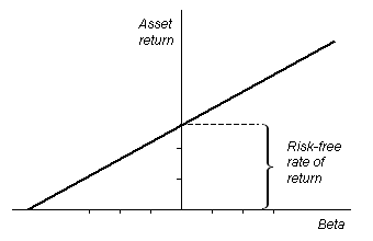
The
Security Market Line, seen here in a graph, describes
a relation between the
beta and the asset's expected rate of return.
|
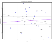
An estimation
of the CAPM and the Security Market Line (purple) for the
Dow Jones Industrial Average over the last 3 years for monthly
data.
The Capital
Asset Pricing Model (CAPM) is used in finance to
determine a theoretically appropriate required rate of return
(and thus the price if expected cash flows can be estimated)
of an asset, if that asset is to be added to an already well-diversified
portfolio, given that asset's non-diversifiable risk. The CAPM
formula takes into account the asset's sensitivity to non-diversifiable
risk (also known as systematic risk or market risk), often represented
by the quantity beta (β) in the financial industry, as well
as the expected return of the market and the expected return
of a theoretical risk-free asset.
The model
was introduced by Jack Treynor, William Sharpe, John Lintner
and Jan Mossin independently, building on the earlier work of
Harry Markowitz on diversification and modern portfolio theory.
Sharpe received the Nobel Memorial Prize in Economics (jointly
with Markowitz and Merton Miller) for this contribution to the
field of financial economics.
The
formula
The CAPM
is a model for pricing an individual security (asset) or a portfolio.
For individual security perspective, we made use of the security
market line (SML) and its relation to expected return and systematic
risk (beta) to show how the market must price individual securities
in relation to their security risk class. The SML enables us
to calculate the reward-to-risk ratio for any security in relation
to that of the overall market. Therefore, when the expected
rate of return for any security is deflated by its beta coefficient,
the reward-to-risk ratio for any individual security in the
market is equal to the market reward-to-risk ratio, thus:
    Individual security’s   / beta    =       Market™s securities (portfolio)
    Reward-to-risk ratio                      Reward-to-risk ratio
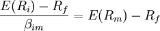 , ,
The market
reward-to-risk ratio is effectively the market risk premium
and by rearranging the above equation and solving for E(Ri),
we obtain the Capital Asset Pricing Model (CAPM).

Where:
 is the expected return on the capital
asset is the expected return on the capital
asset
 is the risk-free rate of interest is the risk-free rate of interest
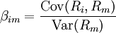
 (the beta coefficient) the
sensitivity of the asset returns to market returns, or also (the beta coefficient) the
sensitivity of the asset returns to market returns, or also
 , ,
 is the expected return of the market is the expected return of the market
 is sometimes known as the market
premium or risk premium (the difference between
the expected market rate of return and the risk-free rate
of return). Note 1: the expected market rate of return is
usually measured by looking at the arithmetic average of the
historical returns on a market portfolio (i.e. S&P 500).
Note 2: the risk free rate of return used for determining
the risk premium is usually the arithmetic average of historical
risk free rates of return and not the current risk free rate
of return. is sometimes known as the market
premium or risk premium (the difference between
the expected market rate of return and the risk-free rate
of return). Note 1: the expected market rate of return is
usually measured by looking at the arithmetic average of the
historical returns on a market portfolio (i.e. S&P 500).
Note 2: the risk free rate of return used for determining
the risk premium is usually the arithmetic average of historical
risk free rates of return and not the current risk free rate
of return.
Asset
pricingOnce the expected return, E(Ri), is calculated using
CAPM, the future cash flows of the asset can be discounted to
their present value using this rate (E(Ri)), to establish the
correct price for the asset.
In theory,
therefore, an asset is correctly priced when its observed price
is the same as its value calculated using the CAPM derived discount
rate. If the observed price is higher than the valuation, then
the asset is overvalued (and undervalued when the observed price
is below the CAPM valuation).
Alternatively,
one can "solve for the discount rate" for the observed price
given a particular valuation model and compare that discount
rate with the CAPM rate. If the discount rate in the model is
lower than the CAPM rate then the asset is overvalued (and undervalued
for a too high discount rate).
Asset-specific
required return
The CAPM
returns the asset-appropriate required return or discount rate
- i.e. the rate at which future cash flows produced by the asset
should be discounted given that asset's relative riskiness.
Betas exceeding one signify more than average "riskiness"; betas
below one indicate lower than average. Thus a more risky stock
will have a higher beta and will be discounted at a higher rate;
less sensitive stocks will have lower betas and be discounted
at a lower rate. The CAPM is consistent with intuition - investors
(should) require a higher return for holding a more risky asset.
Since beta
reflects asset-specific sensitivity to non-diversifiable, i.e.
market risk, the market as a whole, by definition, has a beta
of one. Stock market indices are frequently used as local proxies
for the market - and in that case (by definition) have a beta
of one. An investor in a large, diversified portfolio (such
as a mutual fund) therefore expects performance in line
with the market.
Risk
and diversification
The risk
of a portfolio comprises systematic risk, also known as undiversifiable
risk, and unsystematic risk which is also known as idiosyncratic
risk or diversifiable risk. Systematic risk refers to the risk
common to all securities - i.e. market risk. Unsystematic risk
is the risk associated with individual assets. Unsystematic
risk can be diversified away to smaller levels by including
a greater number of assets in the portfolio (specific risks
"average out"). The same is not possible for systematic risk
within one market. Depending on the market, a portfolio of approximately
30-40 securities in developed markets such as UK or US will
render the portfolio sufficiently diversified to limit exposure
to systemic risk only. In developing markets a larger number
is required, due to the higher asset volatilities.
A rational
investor should not take on any diversifiable risk, as only
non-diversifiable risks are rewarded within the scope of this
model. Therefore, the required return on an asset, that is,
the return that compensates for risk taken, must be linked to
its riskiness in a portfolio context - i.e. its contribution
to overall portfolio riskiness - as opposed to its "stand alone
riskiness." In the CAPM context, portfolio risk is represented
by higher variance i.e. less predictability. In other words
the beta of the portfolio is the defining factor in rewarding
the systematic exposure taken by an investor.
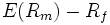
The
efficient frontier
The
(Markowitz) efficient frontier
The CAPM
assumes that the risk-return profile of a portfolio can be optimized
- an optimal portfolio displays the lowest possible level of
risk for its level of return. Additionally, since each additional
asset introduced into a portfolio further diversifies the portfolio,
the optimal portfolio must comprise every asset, (assuming no
trading costs) with each asset value-weighted to achieve the
above (assuming that any asset is infinitely divisible). All
such optimal portfolios, i.e., one for each level of return,
comprise the efficient frontier.
Because
the unsystematic risk is diversifiable, the total risk of a
portfolio can be viewed as beta.
The
market portfolio
An investor
might choose to invest a proportion of his or her wealth in
a portfolio of risky assets with the remainder in cash - earning
interest at the risk free rate (or indeed may borrow money to
fund his or her purchase of risky assets in which case there
is a negative cash weighting). Here, the ratio of risky assets
to risk free asset does not determine overall return - this
relationship is clearly linear. It is thus possible to achieve
a particular return in one of two ways:
- By investing
all of one's wealth in a risky portfolio,
- or by
investing a proportion in a risky portfolio and the remainder
in cash (either borrowed or invested).
For a given
level of return, however, only one of these portfolios will
be optimal (in the sense of lowest risk). Since the risk free
asset is, by definition, uncorrelated with any other asset,
option 2 will generally have the lower variance and hence be
the more efficient of the two.
This relationship
also holds for portfolios along the efficient frontier: a higher
return portfolio plus cash is more efficient than a lower return
portfolio alone for that lower level of return. For a given
risk free rate, there is only one optimal portfolio which can
be combined with cash to achieve the lowest level of risk for
any possible return. This is the market portfolio.
Assumptions
of CAPM
- All investors
have rational expectations.
- There
are no arbitrage opportunities.
- Returns
are distributed normally.
- Fixed
quantity of assets.
- Perfectly
efficient capital markets.
- Investors
are solely concerned with level and uncertainty of future
wealth
- Separation
of financial and production sectors.
- Thus,
production plans are fixed.
- Risk-free
rates exist with limitless borrowing capacity and universal
access.
- The Risk-free
borrowing and lending rates are equal.
- No inflation
and no change in the level of interest rate exists.
- Perfect
information, hence all investors have the same expectations
about security returns for any given time period.
Shortcomings
of CAPM
- The model
assumes that asset returns are (jointly) normally distributed
random variables. It is however frequently observed that returns
in equity and other markets are not normally distributed.
As a result, large swings (3 to 6 standard deviations from
the mean) occur in the market more frequently than the normal
distribution assumption would expect.
- The model
assumes that the variance of returns is an adequate measurement
of risk. This might be justified under the assumption of normally
distributed returns, but for general return distributions
other risk measures (like coherent risk measures) will likely
reflect the investors' preferences more adequately.
- The model
does not appear to adequately explain the variation in stock
returns. Empirical studies show that low beta stocks may offer
higher returns than the model would predict. Some data to
this effect was presented as early as a 1969 conference in
Buffalo, New York in a paper by Fischer Black, Michael Jensen,
and Myron Scholes. Either that fact is itself rational (which
saves the efficient markets hypothesis but makes CAPM wrong),
or it is irrational (which saves CAPM, but makes EMH wrong
indeed, this possibility makes volatility arbitrage a strategy
for reliably beating the market).
- The model
assumes that given a certain expected return investors will
prefer lower risk (lower variance) to higher risk and conversely
given a certain level of risk will prefer higher returns to
lower ones. It does not allow for investors who will accept
lower returns for higher risk. Casino gamblers clearly pay
for risk, and it is possible that some stock traders will
pay for risk as well.
- The model
assumes that all investors have access to the same information
and agree about the risk and expected return of all assets
(homogeneous expectations assumption).
- The model
assumes that there are no taxes or transaction costs, although
this assumption may be relaxed with more complicated versions
of the model.
- The market
portfolio consists of all assets in all markets, where each
asset is weighted by its market capitalization. This assumes
no preference between markets and assets for individual investors,
and that investors choose assets solely as a function of their
risk-return profile. It also assumes that all assets are infinitely
divisible as to the amount which may be held or transacted.
- The market
portfolio should in theory include all types of assets that
are held by anyone as an investment (including works of art,
real estate, human capital...) In practice, such a market
portfolio is unobservable and people usually substitute a
stock index as a proxy for the true market portfolio. Unfortunately,
it has been shown that this substitution is not innocuous
and can lead to false inferences as to the validity of the
CAPM, and it has been said that due to the inobservability
of the true market portfolio, the CAPM might not be empirically
testable. This was presented in greater depth in a paper by
Richard Roll in 1977, and is generally referred to as Roll's
Critique. Theories such as the Arbitrage Pricing Theory (APT)
have since been formulated to circumvent this problem.
- Because
CAPM prices a stock in terms of all stocks and bonds, it is
really an arbitrage pricing model which throws no light on
how a firm's beta is determined.
References
- Black,
Fischer., Michael C. Jensen, and Myron Scholes (1972). The
Capital Asset Pricing Model: Some Empirical Tests, pp.
79-121 in M. Jensen ed., Studies in the Theory of Capital
Markets. New York: Praeger Publishers.
- Fama,
Eugene F. (1968). Risk, Return and Equilibrium: Some Clarifying
Comments. Journal of Finance Vol. 23, No. 1, pp. 29-40.
- Fama,
Eugene F. and Kenneth French (1992). The Cross-Section
of Expected Stock Returns. Journal of Finance, June 1992,
427-466.
- French,
Craig W. (2003). The Treynor Capital Asset Pricing Model,
Journal of Investment Management, Vol. 1, No. 2, pp. 60-72.
Available at http://www.joim.com/
- French,
Craig W. (2002). Jack Treynor's 'Toward a Theory of Market
Value of Risky Assets' (December). Available at http://ssrn.com/abstract=628187
- Lintner,
John (1965). The valuation of risk assets and the selection
of risky investments in stock portfolios and capital budgets,
Review of Economics and Statistics, 47 (1), 13-37.
- Markowitz,
Harry M. (1999). The early history of portfolio theory:
1600-1960, Financial Analysts Journal, Vol. 55, No. 4
- Mehrling,
Perry (2005). Fischer Black and the Revolutionary Idea of
Finance. Hoboken: John Wiley & Sons, Inc.
- Mossin,
Jan. (1966). Equilibrium in a Capital Asset Market,
Econometrica, Vol. 34, No. 4, pp. 768-783.
- Ross,
Stephen A. (1977). The Capital Asset Pricing Model (CAPM),
Short-sale Restrictions and Related Issues, Journal of
Finance, 32 (177)
- Rubinstein,
Mark (2006). A History of the Theory of Investments. Hoboken:
John Wiley & Sons, Inc.
- Sharpe,
William F. (1964). Capital asset prices: A theory of market
equilibrium under conditions of risk, Journal of Finance,
19 (3), 425-442
- Stone,
Bernell K. (1970) Risk, Return, and Equilibrium: A General
Single-Period Theory of Asset Selection and Capital-Market
Equilibrium. Cambridge: MIT Press.
- Tobin,
James (1958). Liquidity preference as behavior towards
risk, The Review of Economic Studies, 25
- Treynor,
Jack L. (1961). Market Value, Time, and Risk. Unpublished
manuscript.
- Treynor,
Jack L. (1962). Toward a Theory of Market Value of Risky
Assets. Unpublished manuscript. A final version was published
in 1999, in Asset Pricing and Portfolio Performance: Models,
Strategy and Performance Metrics. Robert A. Korajczyk (editor)
London: Risk Books, pp. 15-22.
- Mullins,
David W. (1982). Does the capital asset pricing model work?,
Harvard Business Review, January-February 1982, 105-113.
|
|